Contents
An Axes3D object is created just like any other axes using the projection=‘3d’ keyword. Create a new matplotlib.figure.Figure and add a new axes to it of type Axes3D:
import matplotlib.pyplot as plt
from mpl_toolkits.mplot3d import Axes3D
fig = plt.figure()
ax = fig.add_subplot(111, projection='3d')
New in version 1.0.0: This approach is the preferred method of creating a 3D axes.
Note
Prior to version 1.0.0, the method of creating a 3D axes was different. For those using older versions of matplotlib, change ax = fig.add_subplot(111, projection='3d') to ax = Axes3D(fig).
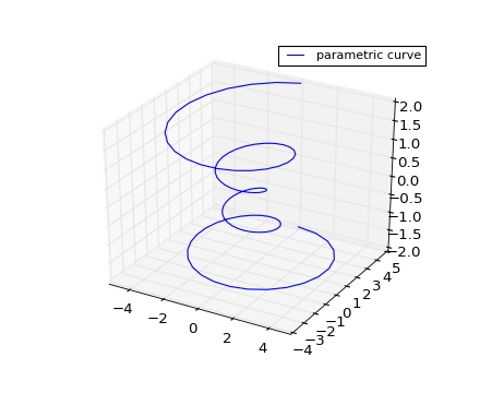
Plot 2D or 3D data.
| Argument | Description |
|---|---|
| xs, ys | X, y coordinates of vertices |
| zs | z value(s), either one for all points or one for each point. |
| zdir | Which direction to use as z (‘x’, ‘y’ or ‘z’) when plotting a 2D set. |
Other arguments are passed on to plot()
(Source code, png)

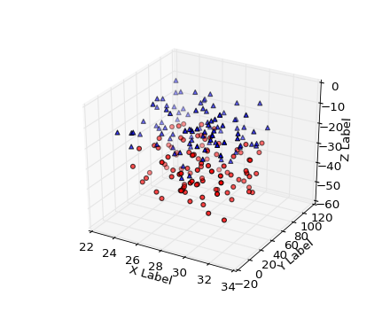
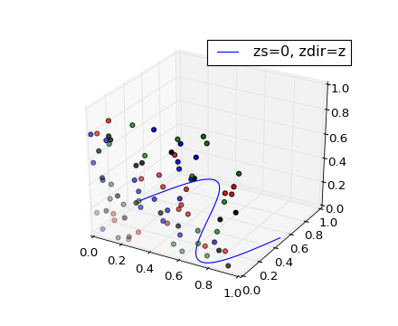
Create a scatter plot.
| Argument | Description |
|---|---|
| xs, ys | Positions of data points. |
| zs | Either an array of the same length as xs and ys or a single value to place all points in the same plane. Default is 0. |
| zdir | Which direction to use as z (‘x’, ‘y’ or ‘z’) when plotting a 2D set. |
| s | size in points^2. It is a scalar or an array of the same length as x and y. |
| c | a color. c can be a single color format string, or a sequence of color specifications of length N, or a sequence of N numbers to be mapped to colors using the cmap and norm specified via kwargs (see below). Note that c should not be a single numeric RGB or RGBA sequence because that is indistinguishable from an array of values to be colormapped. c can be a 2-D array in which the rows are RGB or RGBA, however. |
Keyword arguments are passed on to scatter().
Returns a Patch3DCollection
(Source code, png)

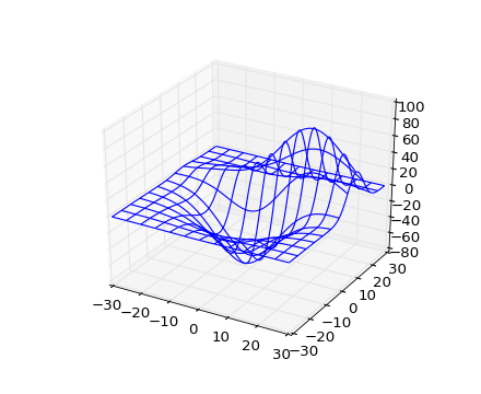
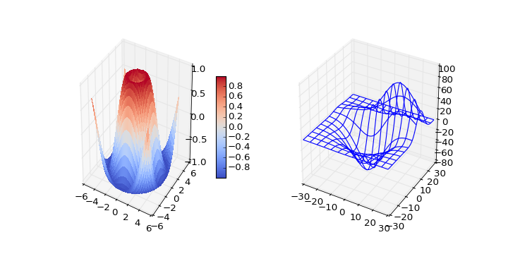
Plot a 3D wireframe.
| Argument | Description |
|---|---|
| X, Y, | Data values as 2D arrays |
| Z | |
| rstride | Array row stride (step size) |
| cstride | Array column stride (step size) |
Keyword arguments are passed on to LineCollection.
Returns a Line3DCollection
(Source code, png)

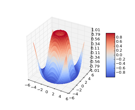
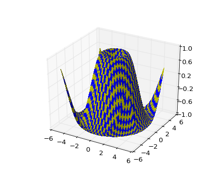
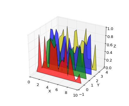
Create a surface plot.
By default it will be colored in shades of a solid color, but it also supports color mapping by supplying the cmap argument.
| Argument | Description |
|---|---|
| X, Y, Z | Data values as 2D arrays |
| rstride | Array row stride (step size) |
| cstride | Array column stride (step size) |
| color | Color of the surface patches |
| cmap | A colormap for the surface patches. |
| facecolors | Face colors for the individual patches |
| norm | An instance of Normalize to map values to colors |
| vmin | Minimum value to map |
| vmax | Maximum value to map |
| shade | Whether to shade the facecolors |
Other arguments are passed on to Poly3DCollection
(Source code, png)

(Source code, png)

(Source code, png)

| Argument | Description |
|---|---|
| X, Y, Z | Data values as 1D arrays |
| color | Color of the surface patches |
| cmap | A colormap for the surface patches. |
| norm | An instance of Normalize to map values to colors |
| vmin | Minimum value to map |
| vmax | Maximum value to map |
| shade | Whether to shade the facecolors |
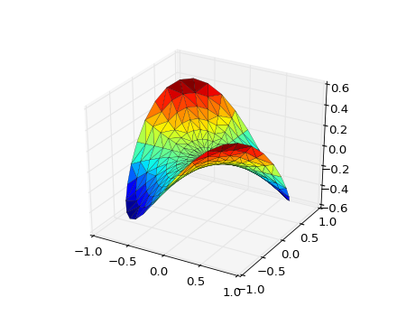
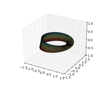
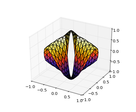
The (optional) triangulation can be specified in one of two ways; either:
plot_trisurf(triangulation, ...)
where triangulation is a Triangulation object, or:
plot_trisurf(X, Y, ...)
plot_trisurf(X, Y, triangles, ...)
plot_trisurf(X, Y, triangles=triangles, ...)
in which case a Triangulation object will be created. See Triangulation for a explanation of these possibilities.
The remaining arguments are:
plot_trisurf(..., Z)
where Z is the array of values to contour, one per point in the triangulation.
Other arguments are passed on to Poly3DCollection
Examples:
(Source code, png)

(png)

(png)
New in version 1.2.0: This plotting function was added for the v1.2.0 release.
(Source code, png)
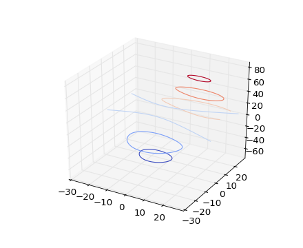
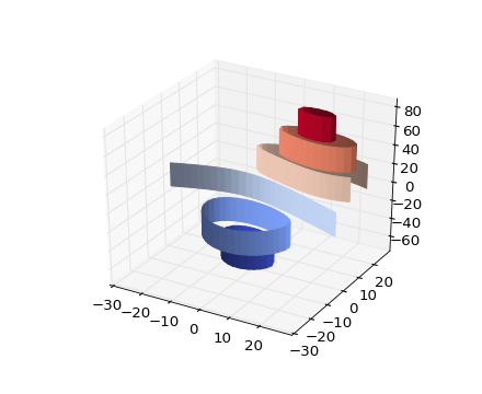
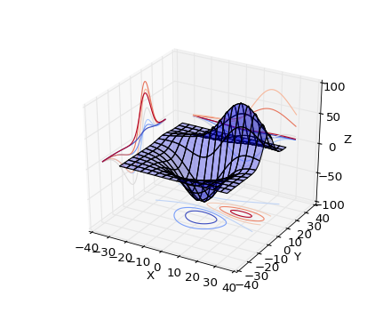
Create a 3D contour plot.
| Argument | Description |
|---|---|
| X, Y, | Data values as numpy.arrays |
| Z | |
| extend3d | Whether to extend contour in 3D (default: False) |
| stride | Stride (step size) for extending contour |
| zdir | The direction to use: x, y or z (default) |
| offset | If specified plot a projection of the contour lines on this position in plane normal to zdir |
The positional and other keyword arguments are passed on to contour()
Returns a contour
(Source code, png)

(Source code, png)

(Source code, png)

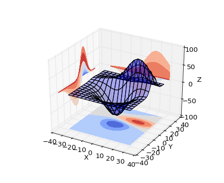
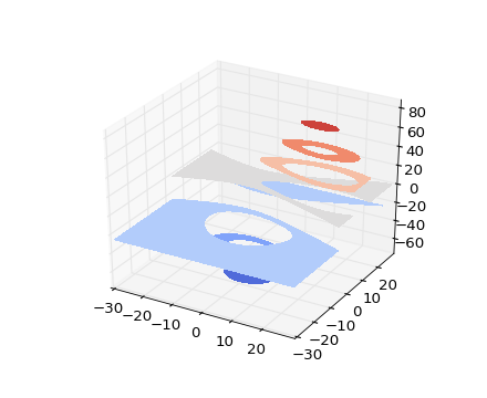
Create a 3D contourf plot.
| Argument | Description |
|---|---|
| X, Y, | Data values as numpy.arrays |
| Z | |
| zdir | The direction to use: x, y or z (default) |
| offset | If specified plot a projection of the filled contour on this position in plane normal to zdir |
The positional and keyword arguments are passed on to contourf()
Returns a contourf
Changed in version 1.1.0: The zdir and offset kwargs were added.
(Source code, png)

(Source code, png)
New in version 1.1.0: The feature demoed in the second contourf3d example was enabled as a result of a bugfix for version 1.1.0.
Add a 3D collection object to the plot.
2D collection types are converted to a 3D version by modifying the object and adding z coordinate information.
(Source code, png)

Add 2D bar(s).
| Argument | Description |
|---|---|
| left | The x coordinates of the left sides of the bars. |
| height | The height of the bars. |
| zs | Z coordinate of bars, if one value is specified they will all be placed at the same z. |
| zdir | Which direction to use as z (‘x’, ‘y’ or ‘z’) when plotting a 2D set. |
Keyword arguments are passed onto bar().
Returns a Patch3DCollection
(Source code, png)

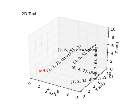
Add text to the plot. kwargs will be passed on to Axes.text, except for the zdir keyword, which sets the direction to be used as the z direction.
(Source code, png)
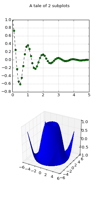
Having multiple 3D plots in a single figure is the same as it is for 2D plots. Also, you can have both 2D and 3D plots in the same figure.
New in version 1.0.0: Subplotting 3D plots was added in v1.0.0. Earlier version can not do this.
(Source code, png)

(Source code, png)


